A Little Gradient Descent

I’ve been increasingly interested in AI, so as an exercise I decided to play around with some simple optimization problems using gradient descent. I really thought I understood gradient descent, but my first attempts to get something working were total failures. For all my theoretical understanding, I didn’t really see how all of the pieces fit together. That, together with some bugs on the part of my autodiff implementation, made for a frustrating morning.

In this note we’ll use gradient descent to train a tiny model to emulate a linear function (an example of a regression problem). We’ll construct the entire system “from scratch”, so we’ll also see how automatic differentation works.

Overview

The GIF above illustrates well what we’re trying to do: the blue line is the linear function we’d like to emulate, and the orange function shows the current behavior of our model as it “learns” the blue line. We’ll view this as an optimization problem in which we want to optimize the “nearness” of the orange line (our model’s behavior) to the blue line. One simple way to measure this nearness is with mean squared error: we pick some x values—say -2 and 3—calculate the value of our “target” line and our model at those points, and combine them like so:

where $T$ is our target function and $M$ is our model.

The key observation here is that the $\mathrm{error}$ is a function of our model’s parameters. Our goal is to find the values of the parameters so that the error is minimized.

Differentiation

Gradient descent attacks this optimization problem by repeatedly calculating little nudges for each parameter’s value. And these updates are based on the derivative of the error with respect to each parameter. So we’re going to need a way to differentiate expressions.

There are many ways to implement automatic differentiation (“autodiff”), but we’ll stick with a really simple approach here. In particular, we’ll create a way to construct symbolic expressions involving numbers, variables, and arithmetic operations. Differentiation is then just a simple recursive process, not too different from evaluation.

We’ll represent expressions using a class Expr, which is a “sum” type having two variants: “symbols” and “binary operations”:

class Expr:
    def sym(name):
        """Construct a symbol, representing a variable."""
        e = Expr()
        e.type = "SYM"
        e.name = name
        return e

    def bin(op, lhs, rhs):
        """Construct an expression representing a binary operation."""
        e = Expr()
        e.type = "BIN"
        e.op = op
        e.lhs = lhs
        e.rhs = rhs
        return e

So Expr.sym('x') creates an expression representing the variable $x$, and Expr.bin('+', Expr.sym('x'), 2)` represents $x + 2$.

So an expression is either an instance of Expr or a Python number.

It will be convenient to be able to unpack Expr instances, so we’ll define __iter__:

def __iter__(self):
    if self.type == "SYM":
        return iter((self.name,))
    elif self.type == "BIN":
        return iter((self.op, self.lhs, self.rhs))

and using our new unpacking ability, we’ll define __str__:

def __str__(self):
    if self.type == "SYM":
        return self.name
    elif self.type == "BIN":
        op, lhs, rhs = self
        return f"({op} {str(lhs)} {str(rhs)})"

This just renders Expr instances as S-Expressions. Let’s see how it works:

x = Expr.sym('x')
y = Expr.sym('y')

e = Expr.bin('+', Expr.bin('**', x, 2), Expr.bin('*', x, y))
print(e)
# => (+ (** x 2) (* x y))

Creating compound expressions using Expr.bin(...) is a pain. Let’s define __add__, __mul__, etc. so that the above expression can be created like:

e = x**2 + x * y

These do nothing more than dispatch to Expr.bin with the appropriate arguments:

def __add__(self, rhs):
    return Expr.bin("+", self, rhs)

def __radd__(self, rhs):
    return Expr.bin("+", rhs, self)

def __mul__(self, rhs):
    return Expr.bin("*", self, rhs)

def __rmul__(self, rhs):
    return Expr.bin("*", rhs, self)

# ...

We’ll also define a convenient way to initialize variables:

def params(names):
    names = names.split(" ")
    if len(names) == 1:
        return Expr.sym(names[0])
    return map(Expr.sym, names)

We can now define the example above very concisely like so:

x, y = params("x y")
e = x**2 + x * y

Our goal is to differentiate expressions like e. This is actually very easy. And that’s because, like evaluation, differentiation has a kind of “compositional” quality to it. What this means is that:

• There are straightforward ways to compute the derivative of “simple” expressions (like variables and numbers).
• In order to compute the derivative of a “compound” expression, you only need to compute the derivatives of its components, and then “glue” them together in some way.

Differentiation as we’ll implement it here is a function of two variables: an expression and a name. The result is the derivative of the expression with respect to the variable with that name.

First, the simple rules for “atomic” expressions:

That is, the derivative of a number with respect to any variable is 0, and the derivative of a variable with respect to another variable is 1 if they’re the same, and 0 if they’re not.

In Python:

def d(e, x):
    """Compute the derivative of the expression e w.r.t. the symbol whose name
    is x."""
    if isinstance(e, Expr):
        if e.type == "SYM":
            return 1 if e.name == x else 0

        elif e.type == "BIN":
            # ...

    else:
        return 0

To compute the derivatives of binary expressions, we need to implement the chain rule. This says that if $e = l \oplus r$, then the derivative of $e$ w.r.t a variable $x$ is:

This is compositionality in action: $\mathrm{d}(l, x)$ and $\mathrm{d}(r, x)$ are just recursive calls to $\mathrm{d}$. $\mathrm{d}_{el}$ and $\mathrm{d}_{er}$ depend on the particular operation $\oplus$. For example, if $e = l + r$, then $\mathrm{d}_{el} = \mathrm{d}_{er} = 1$, whereas if $e = l \cdot r$, then $\mathrm{d}_{el} = r$ and $\mathrm{d}_{er} = l$.

In Python:

def d(e, x):
    if isinstance(e, Expr):
        if e.type == "SYM":
            return 1 if e.name == x else 0

        elif e.type == "BIN":
            op, l, r = e

            dl_dx = d(l, x)
            dr_dx = d(r, x)

            if op == "+":
                de_dl = 1
                de_dr = 1
            if op == "-":
                de_dl = 1
                de_dr = -1
            elif op == "*":
                de_dl = r
                de_dr = l
            elif op == "/":
                de_dl = 1 / r
                de_dr = -l / r**2
            elif op == "**":
                # Only nonnegative integer powers for now:
                de_dl = r * l ** (r - 1)
                de_dr = 0

            return de_dl * dl_dx + de_dr * dr_dx

    else:
        return 0

Let’s try it out:

x, y = params('x y')
e = x**2 + x * y

de_dx = d(e, "x")
# => (+ (* 1 (+ (* (* 2 (** x 1)) 1) 0)) (* 1 (+ (* y 1) (* x 0))))

de_dy = d(e, "y")
# => (+ (* 1 (+ (* (* 2 (** x 1)) 0) 0)) (* 1 (+ (* y 0) (* x 1))))

Yikes! The result returned by d is an unsimplified mess, but it’s nonetheless correct.

Finally, we’re going to need a way to evaluate expressions within some “environment”. Using dicts to represent environments, this is trivial:

def val(e, env):
    """Calculate the value of the expression e in the environment env."""
    if isinstance(e, Expr):
        if e.type == "SYM":
            return env.get(e.name)
        elif e.type == "BIN":
            op, l, r = e
            lv = val(l, env)
            rv = val(r, env)

            if op == "+":
                return lv + rv
            elif op == "-":
                return lv - rv
            elif op == "*":
                return lv * rv
            elif op == "/":
                return lv / rv
            elif op == "**":
                return lv**rv
    else:
        return e

We can now evaluate arbitrary expressions, including the results of differentiation:

env = {"x": 2, "y": 3}

val(e, env)
# => 10

val(de_dx, env)
# => 7

val(de_dy, env)
# => 2

…Back to Optimization

We want to train a model to emulate a linear function. Let’s use:

def target(x):
    return 2 * x + 1

as our target line.

Our model will be a linear function with two parameters: one for the slope and the other for the y-intercept. We define it as a function that returns an expression, which will allow us to differentiate expressions built using it:

m, b = params("m b")

def model(x):
    return m * x + b

Now our goal is to find values for m and b that make model behave like target. Let’s pretend we don’t know any better, and initialize them both to 0:

param_vals = {"m": 0, "b": 0}

We can then evaluate our model at the current parameter values at any input value using val:

def model_val(x):
    e = model(x)
    return val(e, param_vals)

Finally, we’ll need some data to train our model on. For this, we’ll just sample two points using our target line:

train_xs = [-2, 3]
train_ys = [target(x) for x in train_xs]

Recall that we’re trying to optimize the mean squared error of our model w.r.t. the target line. This involves:

1. Applying our model to each $x$ value in the training data.
2. Summing the squared differences between our model’s prediction and the desired $y$-value (and then dividing by the size of the dataset).

predictions = [model(x) for x in train_xs]
loss = sum((pi - yi) ** 2 for pi, yi in zip(predictions, train_ys)) / len(train_xs)

It’s important to note that loss is an expression. Here’s what we get if we print it:

print(loss)
# => (/ (+ (+ 0 (** (- (+ (* m -2) b) -3) 2)) (** (- (+ (* m 3) b) 7) 2)) 2)

As such, we can also differentiate it with respect to our parameters m and b:

dloss_dm = d(loss, 'm')
# => (+ (* 0.5 (+ (* 1 (+ 0 (* 1 (+ (* (* 2 (** (- (+ (* m -2) b) -3) 1)) (+ (* 1 (+ (* 1 (+ -2 (* m 0))) 0)) 0)) 0)))) (* 1 (+ (* (* 2 (** (- (+ (* m 3) b) 7) 1)) (+ (* 1 (+ (* 1 (+ 3 (* m 0))) 0)) 0)) 0)))) (* (/ (- 0 (+ (+ 0 (** (- (+ (* m -2) b) -3) 2)) (** (- (+ (* m 3) b) 7) 2))) 4) 0))

dloss_db = d(loss, 'b')
# => (+ (* 0.5 (+ (* 1 (+ 0 (* 1 (+ (* (* 2 (** (- (+ (* m -2) b) -3) 1)) (+ (* 1 (+ (* 1 (+ 0 (* m 0))) 1)) 0)) 0)))) (* 1 (+ (* (* 2 (** (- (+ (* m 3) b) 7) 1)) (+ (* 1 (+ (* 1 (+ 0 (* m 0))) 1)) 0)) 0)))) (* (/ (- 0 (+ (+ 0 (** (- (+ (* m -2) b) -3) 2)) (** (- (+ (* m 3) b) 7) 2))) 4) 0))

Training

With dloss_dm and dloss_db in hand, training is straightforward. We simply repeat the following steps with both m and b until we’re satisfied with our error:

1. Calculate the derivative of the loss w.r.t. the parameter at the current parameter values.
2. Update the parameter’s value in the direction that decreases the loss (locally); this means moving in the direction opposite the derivative calculated in step (1).

In practice, we don’t update the parameter values in fixed-sized steps, but rather using some fraction of the derivative. This fraction is usually called the learning rate.

Here’s what all this looks like in Python:

# Learning rate and number of training iterations ("hyperparameters").
lr = 0.1
n_iter = 20

for _ in range(n_iter):
    grad_m = val(dloss_dm, param_vals)
    grad_b = val(dloss_db, param_vals)

    param_vals["m"] -= lr * grad_m
    param_vals["b"] -= lr * grad_b

Lo and behold, it works!

Gradient Descent, for Real

What’s different in a real application that uses a standard package like pytorch? The most striking differences are in how the autodiff functionality works. For most interesting applications, the actual derivative expressions would be unthinkably large. The good news is that it’s not necessary to construct these expressions in the first place. That’s because in any given training iteration we’re only interested in the derivative of the loss w.r.t. each parameter at the current parameter values. We’ll go into the details in a future note, but the basic idea is to evaluate the loss expression at the current parameter values, recording the parent-child relationships of the expression in the process. We then calculate derivatives “backwards” from the root of the expression towards the parameters.

This changes the look of our training loop:

for _ in range(n_iter):
    # Run loss function on current parameter values.
    # Backpropagate to calculate gradients.
    # Update parameter values.

A second difference is that in most real applications we don’t consider the entire dataset when calculating the loss, but instead work with batches of the original dataset. This has an important consequence: it means that the loss function being optimized is actually different during different iterations of the training loop.

It also changes our training loop:

# An "epoch" consists of however many training iterations it takes to process
# our training data once.
n_epochs = ...

for epoch in range(n_epochs):
  # E.g. some function that randomly batches all our training data.
  dl = Dataloader(training_data)

  for batch in dl:
      # Calculate loss w.r.t. batch and current parameter values.
      # Backpropagate to calculate gradients.
      # Update parameter values.

A Few More Experiments

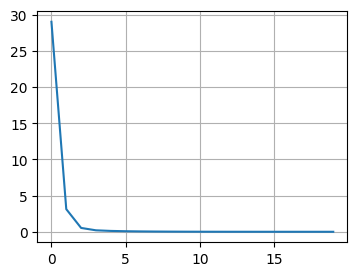
I tried repeating the above experiment with a quadratic function instead of a line. However, I really struggled to get the model to converge, even with more data and more training iterations. Using 3 datapoints:

And 10:

The loss would quickly drop only to bottom out and remain above 0. And if I increased the learning rate I’d run into overflow issues.

I finally logged some of the intermediate parameter values and realized that they had very different “sensitivities”: the same learning rate was causing one to oscillate wildly and another to just plod along. I gave each parameter its own learning rate, tailored to the behavior I observed above, and voila!